Scenario Generation using Bootstrapping
A cornerstone of sensible portfolio management is having a rigid risk management framework in place. So every manager needs a good method to evaluate risk. One such method is scenario generation, which works by creating a set of possible future outcomes for the next time period, with corresponding probabilities.
It is empirically observable that financial markets do not follow a Gaussian stochastic process and sometimes experience losses greater than if returns were normally distributed. Hence, in a portfolio management context it is desirable to manage not only volatility but also tail events – so-called tail scenarios. As the underlying stochastic process is unknown, we need to either assume a probability distribution or to rely on historical observations.
In this post, I will apply bootstrapping of historical returns to create monthly scenarios. Bootstrapping is a non-parametric sampling method similar to Monte-Carlo simulation. The method works by sampling from past observations to generate paths of potential future realizations. The underlying assumption is that the future mimics the past. The financial markets experience strong autocorrelation on a daily frequency, hence, returns are NID (NOT independent and identically distributed). To accommodate this pattern, we resort to block bootstrapping (also known as time-series bootstrapping).
Let’s start by collecting data on S&P 500 and an emerging market index proxied by the ETFs SPY and EEM for the period 2015-01-01 to 2018-12-31. The monthly returns of the ETFs are plotted below.
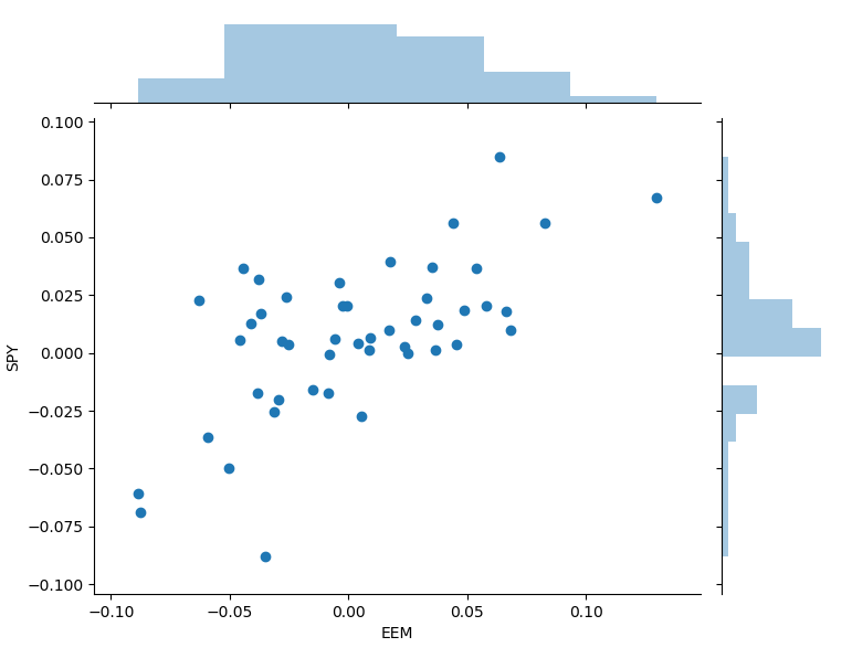
We can observe from the shape of the return distributions (the dots) that the two ETFs are strongly correlated. In addition, there are only 47 dots, so we might not have a good representation of what could happen in a tail scenario.
To get a better understanding of the risk that we undertake, I use block bootstrapping to generate monthly scenarios. This is done by randomly selecting four sequences of five consecutive days from the daily data and then accumulate the returns for these dates to create a monthly realization. We perform this task 1.000 times. We use the same dates for all assets to preserve the correlation between assets, while grouping dates into blocks ensures that we don’t destroy the autocorrelation. The 1.000 scenarios are shown in the following graph.
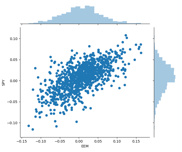
We can observe that there is still strong correlation between the two assets. In addition, we have much more pessimistic scenarios compared to the historic ones without them being too unrealistic.
Long-term and Short-term Tail Scenarios
When sampling from historical data, we have assumed so far that data from 3 years ago is equally relevant as data from yesterday. This is probably not true in reality, as the current economic situation might be vastly different from the one three years ago. Hence, we should put more weight on newer data.
We modify the block bootstrap model a bit, so that we sample from a truncated normal distribution instead of a uniform distribution. The truncated normal distribution is basically the left side of the normal distribution, and looks like this.
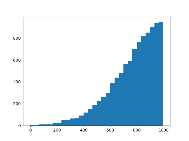
If we use this distribution instead, then we get more samples from the newest data and less from the oldest data, though some older realizations are still included. Again, we generate 1.000 monthly scenarios and plot the results.
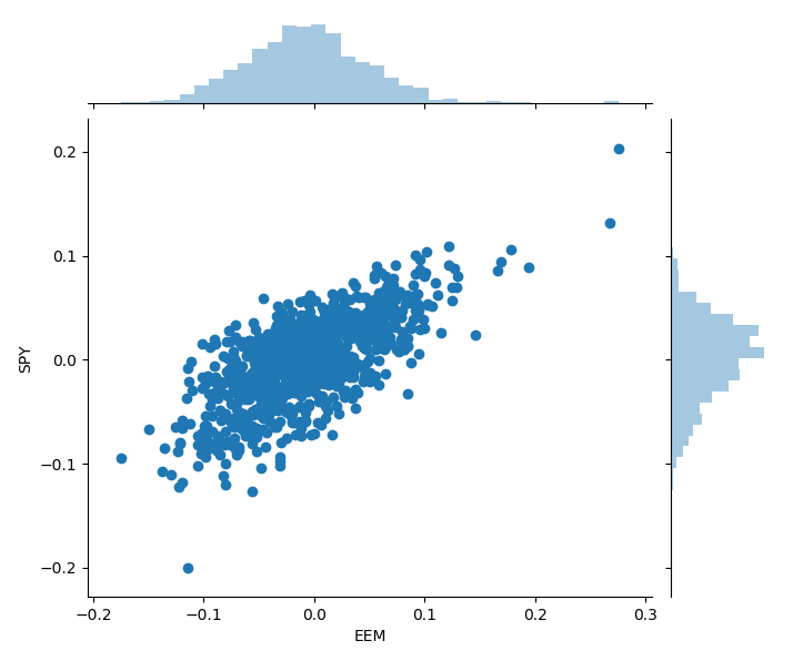
We see that we get even more extreme scenarios using this method. If we remember back to the end of 2018, then the stock markets had been through a very turbulent period of several ups and down, e.g. the U.S. stocks had their worst year in a decade with a loss of more than 6%. These losses are directly reflected in the scenarios which give a much better representation of the risk than the original historical returns.
Scenario generation is not only usefull for understanding the risk of a single asset, but can also be directly applied in a portfolio optimization setting. For example, optimizing a portfolio using the CVaR risk measure requires a good representation of the non-normal risk distribution. The scenario generation can be successfully applied in this case to provide such distribution.
Code
Download of Data and CVaR Optimization
# We would like all available data from 01/01/2000 until 12/31/2016.
start_date = '2015-01-01'
end_date = '2018-12-31'

# tickers
tickers = ["SPY","EEM"]

# User pandas_reader.data.DataReader to load the desired data.
panel_data = data.DataReader(tickers, 'yahoo', start_date, end_date)
df_close = panel_data["Adj Close"]

# Daily returns, and remove the first row as it is NA
df_ret = df_close.pct_change().iloc[1:]

# ini boot
Boot = Bootstrapping()

# Block bootstrapping
BBscen = Boot.BBscenario(dat_avail=df_ret)

# block bootstrapping using truncated normal
BBtail = Boot.BBscenario_sequential(dat_avail=df_ret)


# plot truncated normal distribution
n_ahead = 20
block_size = 5
mean = df_ret.shape[0]-block_size
sd = np.std(range(mean))
low = 0
upp = mean
random.seed(2019)

# plot truncated normal distribution
tcn = truncnorm((low - mean) / sd, (upp - mean) / sd, loc=mean, scale=sd)
t_bars = tcn.rvs( 10000 ).astype(int)
plt.hist(t_bars,bins=30)

## plot block bootstrapped scenarios
sns.jointplot(x="EEM", y="SPY", data=BBscen)

## plot truncated block bootstrapped scenarios
sns.jointplot(x="EEM", y="SPY", data=BBtail)
Functions for Scenario Generation
import pandas as pd
import numpy as np
from pandas_datareader import data
import random
from scipy.stats import truncnorm
import seaborn as sns
import matplotlib.pyplot as plt

class Bootstrapping:

    def BBpath(self,dat_avail,block_size=5,n_ahead=20):
        """
        Generate block boostrapped path "n_ahead" into the future
        """

        draws = random.sample(range(0, dat_avail.shape[0]-block_size), int(np.ceil(n_ahead/block_size)) )

        path = pd.DataFrame(index=range( block_size*int(np.ceil(n_ahead/block_size)) ),columns=dat_avail.columns)
        for i in range(len(draws)):
            path.iloc[(i*block_size): ((i+1)*block_size)] = dat_avail.iloc[draws[i]:(draws[i]+block_size) ].values

        # take the n_ahead vector and save it
        scen_out = (1+path).cumprod(axis=0).iloc[-1]-1

        return scen_out.values

    def BBscenario(self,dat_avail,no_scen=1000,block_size=5,n_ahead=20,para_window=(3*253)):
        """
        Block boostrapping using a normal for-loop
        """

        # reduce data set to only include specific window of data
        dat_avail = dat_avail.iloc[(-para_window):-1 ]

        scen = pd.DataFrame(0,columns=dat_avail.columns,index=range(no_scen))

        for j in range(no_scen):
            scen.iloc[j] = self.BBpath(dat_avail)

        return(scen)


    def get_truncated_normal(self,mean=0, sd=1, low=0, upp=10):
        """
        Generate truncated normal distribution function
        """
        return(truncnorm((low - mean) / sd, (upp - mean) / sd, loc=mean, scale=sd))


    def BBpath_normal(self,dat_avail,block_size=5,n_ahead=20):
        """
        Generate block boostrapped path "n_ahead" into the future
        """

        mean = dat_avail.shape[0]-block_size
        std = np.std(range(mean)) #mean*sd_fraction
        random.seed(2019)

        normal = self.get_truncated_normal(mean=mean, sd=std, low=0, upp=mean)
        draws = normal.rvs( int(np.ceil(n_ahead/block_size)) ).astype(int)

        path = pd.DataFrame(index=range( block_size*int(np.ceil(n_ahead/block_size)) ),columns=dat_avail.columns,data=0.0)

        for i in range(len(draws)):
            path.iloc[(i*block_size): ((i+1)*block_size)] = dat_avail.iloc[draws[i]:(draws[i]+block_size) ].values

        scen_out = (1+path).cumprod()-1

        return(scen_out.iloc[n_ahead-1])


    def BBscenario_sequential(self,dat_avail,no_scen=1000,block_size=5,n_ahead=20,para_window=(3*253)):
        """
        Block boostrapping using a normal for-loop
        """

        # reduce data set to only include specific window of data
        dat_avail = dat_avail.iloc[(-para_window):-1 ]

        scen = pd.DataFrame(columns=dat_avail.columns)

        for j in range(no_scen):
            scen = scen.append(self.BBpath_normal(dat_avail), ignore_index=True)

        return(scen)