Fractional Portfolio Optimization
Asset managers often wish to find the portfolio with the highest risk-adjusted return, as it can leveraged (or de-leveraged) to obtain superior returns compared to any other portfolio. I showed in link how to find this portfolio by solving a portfolio optimization problem for different risk aversion coefficients. This post describes how to find the optimal tangency portfolio in a faster way than previously shown.
Instead of solving the portfolio optimization model over and over for different risk averision coefficients to find the portfolio with the highest risk-adjusted return, we can actually find the optimal portfolio in one step. This can be done using a technique called fractional programming. The method works by mapping the problem into another space and introducing an auxiliary variable . However, certain requirements need to be satisfied before using this approach. We need two objectives, where one seeks to maximize a concave function and another - to miminize a convex function. This is the case for portfolio optimization where we maximize returns (concave) and minimize risk (convex).
If we use the mean-CVaR, we can write the fractional formulation of the model as
where is the fraction to be invested in each asset, and and is the expected return of each asset and a benchmark, respectively. is the Value at Risk, is an auxilirary variable, and is the scenarios.
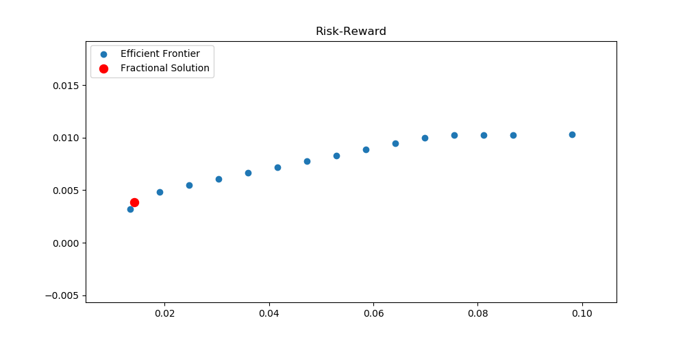
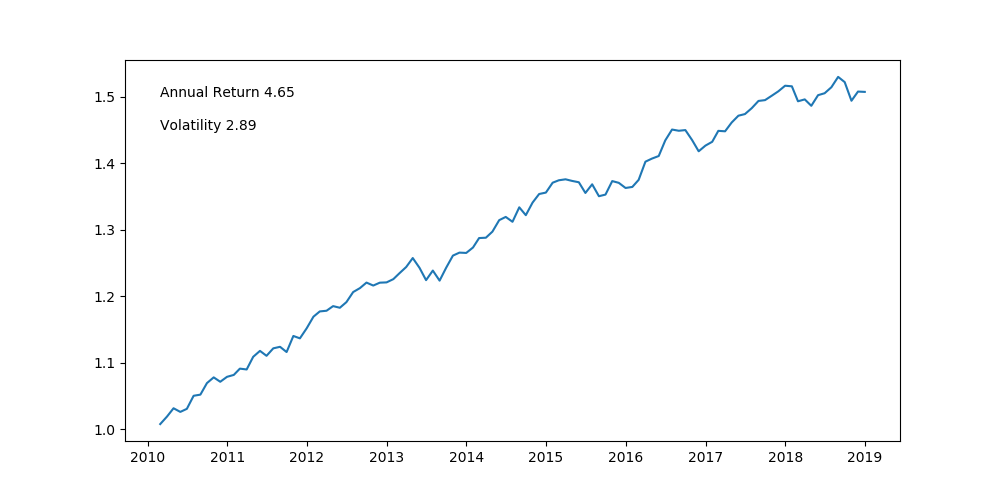
If we use the efficient frontier and compute the optimal fractional portfolio with a benchmark of 0% return, we can observe that that it lies very much to the left on the risk scale. The portfolio consists of 82% bonds, 15% S&P500 and 3% Small Cap, so it is a very risk-averse portfolio.
Historically, this portfolio has performed like this.
Now, if we instead define the benchmark as the 1/N portfolio, which equally weights the different assets, then the historical performance looks like this.
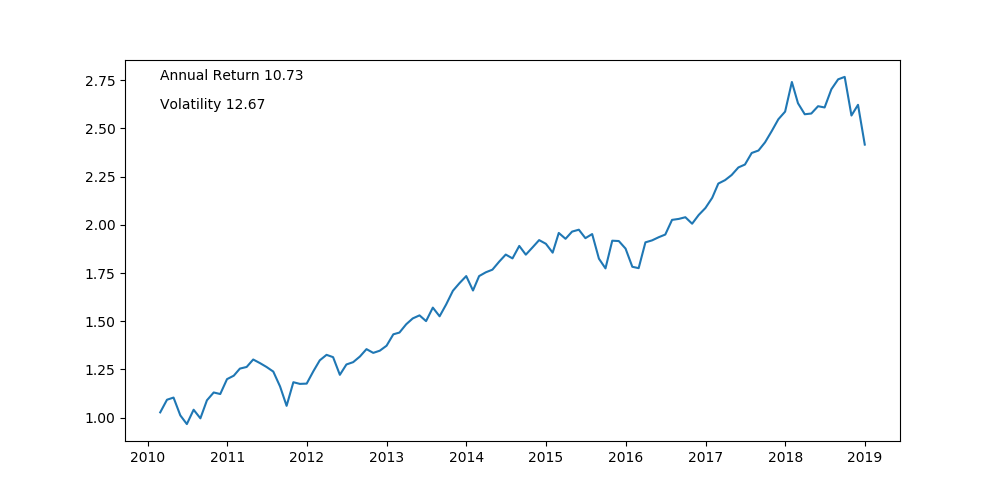
Here, the portfolio consist of 80% S&P 500, 13% Emerging Market and 7% in global Large Cap, excluding the US and Canada.
The benchmark in the model can be seen as a return requirement, and the optimal portfolio is a portfolio which is most likely to outperform it. In this way, the fractional mean-CVaR model can actually be considered as a form of enhanced index tracking, where we seek to construct a model which tracks some index (the benchmark), but also seeks to outperform it.
So far, we have not introduced the leverage into the model. The first portfolio has much higher risk-adjusted returns than the second one, which means that it can be leveraged to deliver superior returns with the same amount of risk, assuming that it is free to borrow money. We need to leverage the first portfolio approximately 4x to obtain the same amount of risk as the second one.
If we construct an insample horse race between the two strategies where the strategies has equal risk, we get the following
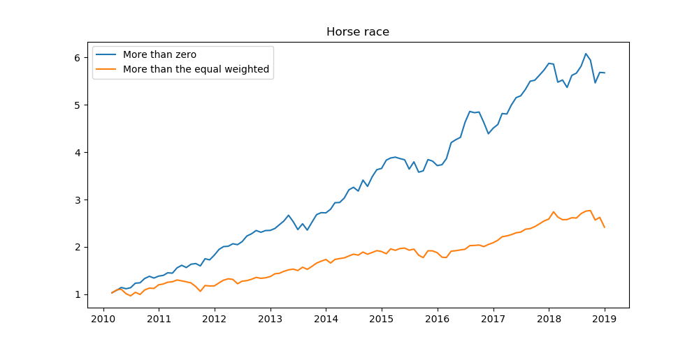
It can be observed that we can greatly outperform the stock heavy portfolio using a very low risk bond heavy portfolio when applying leverage. This is assuming that we don’t have to pay for our financing. In reality, leverage is not free but when applied under the right curcumstances can lead to enhanced absolute and risk adjusted returns.
Code
Download of Data and CVaR Optimization
import pulp
import pandas as pd
import numpy as np
from pandas_datareader import data

# We would like all available data from 01/01/2000 until 12/31/2016.
start_date = '2010-01-01'
end_date = '2018-12-31'

# tickers
tickers = ["SPY","IJS","EFA","EEM","AGG"]

# User pandas_reader.data.DataReader to load the desired data.
panel_data = data.DataReader(tickers, 'yahoo', start_date, end_date)
df_close = panel_data["Adj Close"]

# monthly returns from daily prices, and remove the first row as it is NA
df_ret = df_close.resample('M').last().pct_change().iloc[1:]

#%% compute the optimal portfolio outperforming zero percentage return

mu = df_ret.mean()
mu_b = 0
scen = df_ret
scen_b = pd.Series(0,index=df_ret.index)
min_weight = 0
cvar_alpha=0.05
OptPort_zero = MeanCVaR(mu,mu_b,scen,scen_b,max_weight=1,min_weight=None,cvar_alpha=cvar_alpha)
Functions for CVaR Optimization
#%% packages

import pulp
import pandas as pd
import numpy as np
from pandas_datareader import data


#%% functions


def MeanCVaR(mu,mu_b,scen,scen_b,max_weight=1,min_weight=None,cvar_alpha=0.05):

    """ This function finds the optimal enhanced index portfolio according to some benchmark. The portfolio corresponds to the tangency portfolio where risk is evaluated according to the CVaR of the tracking error. The model is formulated using fractional programming.

    Parameters
    ----------
    mu : pandas.Series with float values
        asset point forecast
    mu_b : pandas.Series with float values
        Benchmark point forecast
    scen : pandas.DataFrame with float values
        Asset scenarios
    scen_b : pandas.Series with float values
        Benchmark scenarios
    max_weight : float
        Maximum allowed weight
    cvar_alpha : float
        Alpha value used to evaluate Value-at-Risk one
    min_val : float
        Values less than this are set to zero. This is used to eliminate floating points


    Returns
    -------
    float
        Asset weights in an optimal portfolio

    Notes
    -----
    The tangency mean-CVaR portfolio is effectively optimized as:
        .. math:: STARR(w) = frac{w^T*mu - mu_b}{CVaR(w^T*scen - scen_b)}
    This procedure is described in [1]_

    References
    ----------
        .. [1] Stoyanov, Stoyan V., Svetlozar T. Rachev, and Frank J. Fabozzi. "Optimal financial portfolios." Applied Mathematical Finance 14.5 (2007): 401-436.

    Examples
    --------
    >>> import pandas as pd
    >>> import numpy as np
    >>> mean = (0.08, 0.09)
    >>> cov = [[0.19, 0.05], [0.05, 0.18]]
    >>> scen = pd.dataframe(np.random.multivariate_normal(mean, cov, 100))
    >>> portfolio = IndexTracker(pd.Series(mean), pd.Series(0), pd.dataframe(scen),pd.Series(0,index=scen.index) )
    """


    # define index
    i_idx = mu.index
    j_idx = scen.index

    # number of scenarios
    N = scen.shape[0]
    M = 100000 # large number

    # define variables
    x = pulp.LpVariable.dicts("x", ( (i) for i in i_idx ),
                                         lowBound=0,
                                         cat='Continuous')

    # loss deviation
    VarDev = pulp.LpVariable.dicts("VarDev", ( (t) for t in j_idx ),
                                         lowBound=0,
                                         cat='Continuous')

    # scaling variable used by fractional programming formulation
    Tau = pulp.LpVariable("Tau",   lowBound=0,
                                         cat='Continuous')

    # value at risk
    VaR = pulp.LpVariable("VaR",   lowBound=0,
                                         cat='Continuous')

    b_z = pulp.LpVariable.dicts("b_z",   ( (i) for i in i_idx ),
                                         cat='Binary')

    # auxiliary to make a non-linear formulation linear (see Linear Programming Models based on Omega Ratio for the Enhanced Index Tracking Problem)
    Tau_i = pulp.LpVariable.dicts("Tau_i", ( (i) for i in i_idx ),
                                         lowBound=0,
                                         cat='Continuous')


    #####################################
    ## define model
    model = pulp.LpProblem("Enhanced Index Tracker (STAR ratio)", pulp.LpMaximize)

    #####################################
    ## Objective Function

    model += pulp.lpSum([mu[i] * x[i] for i in i_idx] ) - Tau*mu_b

    #####################################
    # constraint

    # calculate CVaR
    for t in j_idx:
        model += -pulp.lpSum([ scen.loc[t,i]  * x[i] for i in i_idx] ) + scen_b[t]*Tau - VaR <= VarDev[t]

    model += VaR + 1/(N*cvar_alpha)*pulp.lpSum([ VarDev[t] for t in j_idx]) <= 1

    ### price*number of products cannot exceed budget
    model += pulp.lpSum([ x[i] for i in i_idx]) == Tau

    ### Concentration limits
    # set max limits so it cannot not be larger than a fixed value
    ###
    for i in i_idx:
        model += x[i] <= max_weight*Tau

    ### Add minimum weight constraint, either zero or atleast minimum weight
    if min_weight is not None:

        for i in i_idx:
            model += x[i] >= min_weight*Tau_i[i]
            model += x[i] <= max_weight*Tau_i[i]
            model += Tau_i[i] <= M*b_z[i]
            model += Tau_i[i] <= Tau
            model += Tau - Tau_i[i] + M*b_z[i] <= M


    # solve model
    model.solve(pulp.PULP_CBC_CMD(maxSeconds=60, msg=1, fracGap=0))

    # print an error if the model is not optimal
    if pulp.LpStatus[model.status] != 'Optimal':
        print("Whoops! There is an error! The model as error status:" + pulp.LpStatus[model.status] )


    #Get positions
    if pulp.LpStatus[model.status] == 'Optimal':

        # print variables
        var_model = dict()
        for variable in model.variables():
            var_model[variable.name] = variable.varValue

        # solution with variable names
        var_model = pd.Series(var_model,index=var_model.keys())


        long_pos = [i for i in var_model.keys() if i.startswith("x") ]

        # total portfolio with negative values as short positions
        port_total = pd.Series(var_model[long_pos].values ,index=[t[2:] for t in var_model[long_pos].index])

        # value of tau
        tau_val = var_model[var_model.keys() == 'Tau']

        opt_port = port_total/tau_val[0]
        opt_port[opt_port < 0.00001] = 0 # get rid of floating numbers

    return opt_port