Portfolio Optimization using Conditional Value at Risk
Constructing a portfolio with high risk-adjusted returns is all about risk management. Here, the mitigration of large losses is of paramount importance, as gains and losses are asymmetric by nature. For example, if a portfolio value drops by 10% then we would need to regain 11.1% to neutralize this loss. This post is about how to use the Conditional Value at Risk measure in a portfolio optimization framework.
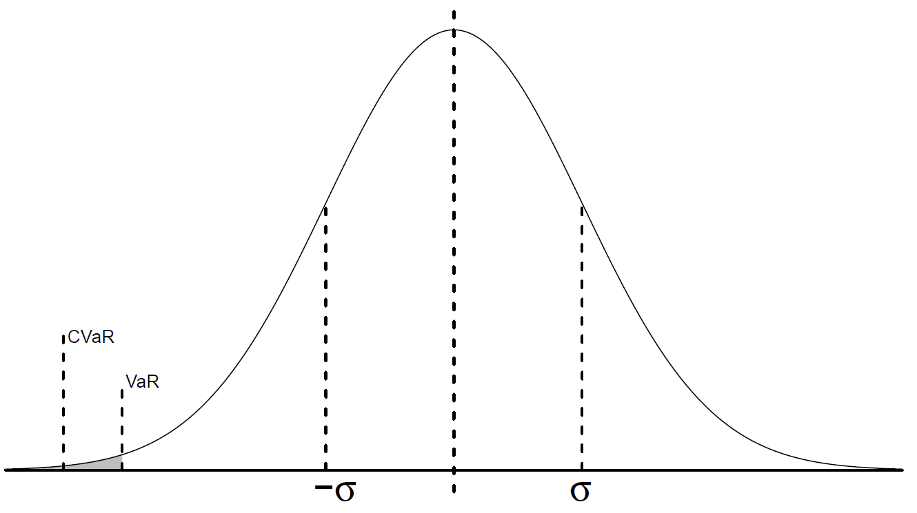
Conditional Value at Risk (CVaR) is a popular risk measure among professional investors used to quantify the extent of potential big losses. The metric is computed as an average of the % worst case scenarios over some time horizon. The measure is a natural extention of the Value at Risk (VaR) proposed in the Basel II Accord.
The introduction of CVaR is justified by many numerical problems of using VaR in practice, e.g. the nessesity to assume normally distributed returns. In addition, the VaR measurement fails to be risk-coherent as it lacks subadditivity and convexity. Here, subadditivity means that a portfolio’s risk cannot exceed the combined risks of the individual positions. In some special cases for the VaR metric, this statement becomes violated and it becomes mathematically possible to obtain a risk reduction by dividing a portfolio into two sub-portfolios. Intuitively, this does not make any sense and breaks the reason for diversifying a portfolio.
So, Conditional Value at Risk is a superior measure of risk and can be mathematically expressed as defined as This can also be visualized like this:
Conditional Value at Risk is not only convinient as it better identifies the tail risk than VaR, but it also holds desirable numerical properties such as linearity. This means that we can easily integrate it in a portfolio optimization framework.
Similar to the mean-variance model, we can construct a portfolio, which maximizes the expected return for some level of risk (in this case, expressed using CVaR).
If we introduce a risk aversion coefficient , then the mean-CVaR portfolio optimisation model can be written:
There exist a quadratic relationship between risk and expected return. Hence, increasing the riskiness of a portfolio will not nessecarily result in an equal increase in expected returns. This is represented by the shape of the efficient frontier.
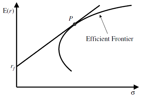
As risk and return are not linearly dependant, it makes sense to consider the marginal increase in expected return when increasing the risk. This effectively leads to the maximization of the Sharpe ratio in the mean-variance setting, and the STAR ratio for CVaR.
The Efficient Frontier
To illustrate the application of CVaR in a portfolio setting, I download data from Yahoo on 5 ETFs, tracking four equity markets and one aggregated bond market respectively. I use the brilliant Python library PuLP to formulate a linear optimization model, and iteratively find the optimal portfolio for different risk aversions, .
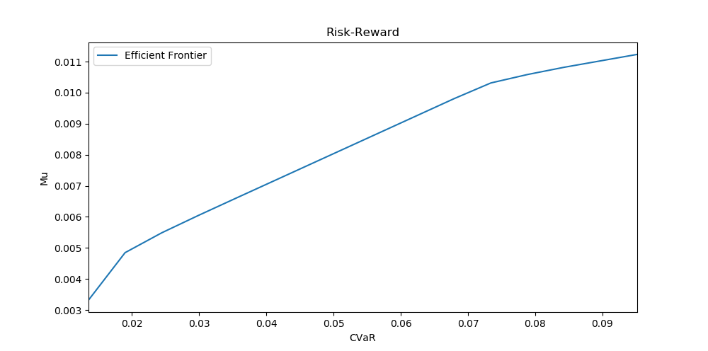 We can observe that our efficient frontier looks similar to what we would expect. In the beginning, we have a large increase in return when allowing for a bit more risk, while in the end we gain nearly no increase in expected returns for the same increase in risk.
Let’s now observe the portfolio allocation for each frontier point.
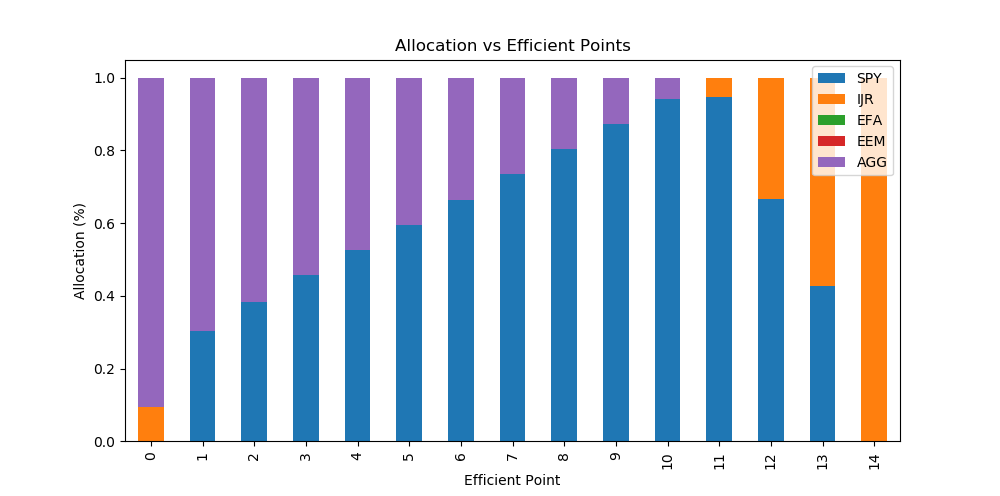
We see that the most risk-averse portfolio consists primarily of bonds with a minor allocation to Small Cap stocks. As we increase the risk level, the equity allocation increases as well. In the beginning, we primarily allocate to the US Large Cap equity, which then changes to the US Small Cap towards the more risky portfolios. This all makes perfect sense according to the economic theory, as bonds should provide the most defensive allocation. Small Cap on average returns higher profits than Large Cap, but also contributes with an additional risk to the portfolio, due to illiquidity, poor capitalisation etc. This is known as the Size risk premia. Interestingly, we can see that our most risk-averse portfolio consist of BOTH bonds and Small Cap. Small Cap should be the most risky investment, but due to the low correlation between bond returns and Small Cap stock returns then we can achieve diversification benefits from including it which more than offset its component risk.
Code
Download of Data and CVaR Optimization
# We download closing prices for the period 01/01/2000 to 12/31/2016.
start_date = '2010-01-01'
end_date = '2018-12-31'

# tickers
tickers = ["SPY","IJS","EFA","EEM","AGG"]

# User pandas_reader.data.DataReader to load the desired data.
panel_data = data.DataReader(tickers, 'yahoo', start_date, end_date)
df_close = panel_data["Adj Close"]

# monthly returns from daily prices, and remove the first row as it is NA
df_ret = df_close.resample('M').last().pct_change().iloc[1:]

#%% compute the optimal portfolio outperforming zero percentage return

mu = df_ret.mean()
scen = df_ret
min_weight = 0
cvar_alpha=0.05
Frontier_port = PortfolioLambda(mu,scen,max_weight=1,min_weight=None,cvar_alpha=cvar_alpha)
Functions for CVaR Optimization
#%% packages

import pulp
import pandas as pd
import numpy as np
from pandas_datareader import data


#%% functions

def PortfolioRiskTarget(mu,scen,CVaR_target=1,lamb=1,max_weight=1,min_weight=None,cvar_alpha=0.05):

    """ This function finds the optimal enhanced index portfolio according to some benchmark. The portfolio corresponds to the tangency portfolio where risk is evaluated according to the CVaR of the tracking error. The model is formulated using fractional programming.

    Parameters
    ----------
    mu : pandas.Series with float values
        asset point forecast
    mu_b : pandas.Series with float values
        Benchmark point forecast
    scen : pandas.DataFrame with float values
        Asset scenarios
    scen_b : pandas.Series with float values
        Benchmark scenarios
    max_weight : float
        Maximum allowed weight
    cvar_alpha : float
        Alpha value used to evaluate Value-at-Risk one

    Returns
    -------
    float
        Asset weights in an optimal portfolio

    """

    # define index
    i_idx = mu.index
    j_idx = scen.index

    # number of scenarios
    N = scen.shape[0]

    # define variables
    x = pulp.LpVariable.dicts("x", ( (i) for i in i_idx ),
                                         lowBound=0,
                                         cat='Continuous')

    # loss deviation
    VarDev = pulp.LpVariable.dicts("VarDev", ( (t) for t in j_idx ),
                                         lowBound=0,
                                         cat='Continuous')

    # value at risk
    VaR = pulp.LpVariable("VaR",   lowBound=0,
                                         cat='Continuous')
    CVaR = pulp.LpVariable("CVaR",   lowBound=0,
                                         cat='Continuous')

    # binary variable connected to cardinality constraints
    b_z = pulp.LpVariable.dicts("b_z",   ( (i) for i in i_idx ),
                                         cat='Binary')

    #####################################
    ## define model
    model = pulp.LpProblem("Mean-CVaR Optimization", pulp.LpMaximize)

    #####################################
    ## Objective Function

    model += lamb*(pulp.lpSum([mu[i] * x[i] for i in i_idx] )) - (1-lamb)*CVaR

    #####################################
    # constraint

    # calculate CVaR
    for t in j_idx:
        model += -pulp.lpSum([ scen.loc[t,i]  * x[i] for i in i_idx] ) - VaR <= VarDev[t]

    model += VaR + 1/(N*cvar_alpha)*pulp.lpSum([ VarDev[t] for t in j_idx]) == CVaR

    model += CVaR <= CVaR_target

    ### price*number of products cannot exceed budget
    model += pulp.lpSum([ x[i] for i in i_idx]) == 1

    ### Concentration limits
    # set max limits so it cannot not be larger than a fixed value
    ###
    for i in i_idx:
        model += x[i] <= max_weight

    ### Add minimum weight constraint, either zero or atleast minimum weight
    if min_weight is not None:

        for i in i_idx:
            model += x[i] >= min_weight*b_z[i]
            model += x[i] <= b_z[i]

    # solve model
    model.solve()

    # print an error if the model is not optimal
    if pulp.LpStatus[model.status] != 'Optimal':
        print("Whoops! There is an error! The model has error status:" + pulp.LpStatus[model.status] )


    #Get positions
    if pulp.LpStatus[model.status] == 'Optimal':

        # print variables
        var_model = dict()
        for variable in model.variables():
            var_model[variable.name] = variable.varValue

        # solution with variable names
        var_model = pd.Series(var_model,index=var_model.keys())


        long_pos = [i for i in var_model.keys() if i.startswith("x") ]

        # total portfolio with negative values as short positions
        port_total = pd.Series(var_model[long_pos].values ,index=[t[2:] for t in var_model[long_pos].index])

        opt_port = port_total

    # set flooting data points to zero and normalize
    opt_port[opt_port < 0.000001] = 0
    opt_port = opt_port/sum(opt_port)

    # return portfolio, CVaR, and alpha
    return opt_port, var_model["CVaR"], (sum(mu * port_total) - mu_b)


def PortfolioLambda(mu,mu_b,scen,scen_b,max_weight=1,min_weight=None,cvar_alpha=0.05,ft_points=15):

    # asset names
    assets = mu.index

    # column names
    col_names = mu.index.values.tolist()
    col_names.extend(["Mu","CVaR","STAR"])
    # number of frontier points


    # store portfolios
    portfolio_ft = pd.DataFrame(columns=col_names,index=list(range(ft_points)))

    # maximum risk portfolio
    lamb=0.99999
    max_risk_port, max_risk_CVaR, max_risk_mu = PortfolioRiskTarget(mu=mu,scen=scen,CVaR_target=100,lamb=lamb,max_weight=max_weight,min_weight=min_weight,cvar_alpha=cvar_alpha)
    portfolio_ft.loc[ft_points-1,assets] = max_risk_port
    portfolio_ft.loc[ft_points-1,"Mu"] = max_risk_mu
    portfolio_ft.loc[ft_points-1,"CVaR"] = max_risk_CVaR
    portfolio_ft.loc[ft_points-1,"STAR"] = max_risk_mu/max_risk_CVaR

    # minimum risk portfolio
    lamb=0.00001
    min_risk_port, min_risk_CVaR, min_risk_mu= PortfolioRiskTarget(mu=mu,scen=scen,CVaR_target=100,lamb=lamb,max_weight=max_weight,min_weight=min_weight,cvar_alpha=cvar_alpha)
    portfolio_ft.loc[0,assets] = min_risk_port
    portfolio_ft.loc[0,"Mu"] = min_risk_mu
    portfolio_ft.loc[0,"CVaR"] = min_risk_CVaR
    portfolio_ft.loc[0,"STAR"] = min_risk_mu/min_risk_CVaR

    # CVaR step size
    step_size = (max_risk_CVaR-min_risk_CVaR)/ft_points # CVaR step size

    # calculate all frontier portfolios
    for i in range(1,ft_points-1):
        CVaR_target = min_risk_CVaR + step_size*i
        i_risk_port, i_risk_CVaR, i_risk_mu= PortfolioRiskTarget(mu=mu,scen=scen,CVaR_target=CVaR_target,lamb=1,max_weight=max_weight,min_weight=min_weight,cvar_alpha=cvar_alpha)
        portfolio_ft.loc[i,assets] = i_risk_port
        portfolio_ft.loc[i,"Mu"] = i_risk_mu
        portfolio_ft.loc[i,"CVaR"] = i_risk_CVaR
        portfolio_ft.loc[i,"STAR"] = i_risk_mu/i_risk_CVaR

    return portfolio_ft